pore network model

Network modelling of porous and confined media

Background

The classical network flow simulation code called poreflow was originally developed by Valvatne and Blunt(2004). Later on, a network extraction code has been developed by Dong and Blunt, 2009.

These codes were further improved and released on Github in a single git submodule called PNM; see code. These codes were further developed for generalized network extraction and generalized network flow modeling, together called GNM.

Similar to GNM, the snflow and snextract code, collectively called SNM, are revised and extended versions of the pnextract and pnflow codes, aiming to improve their accuracy, performance and scope. This is achieved through the use of a Xdmf surface format to preserve the information obtained during medial-surface extraction from the underlying image. Additionally, SNM codes treat the geometry as a stochastic network model description to deal with the input micro-CT image uncertainty. Furthermore a multi-region network extraction adds support for Darcy-based flow models that allows modeling flow through unresolved (usually nano-scale) pores that are coupled with the flow through larger micro-scale pores and throats.

snextract

The input file format for snextract is any image supported by libvoxel, or directly on a .tif image or Avizo file with suffix .am. The output of snextract (and input of snflow) is a file based on Xdmf file format, which can directly be visualized in Paraview software.

Snextract and snflow are however, are primarily invoked through the sirun C++ or Python workflows, where the input data are provided as Json-like dictionaries.

Additional image processing commands, (see libvoxel/voxelImageProcess documentation) can be given immediately after the above keywords, or as arguments to a VxlPro keyword enclosed by brackets.

VxlPro: {
    crop: 0 0 0 200 200 200;
    # Cut out a cylinder of radius 450 voxels, centred at x=500,y=500:
    circleOut: z 500 500  450
    redirect: z # flip x and z directions.
}

Medial-surface settings (optional)

The medialSurfaceSettings is an optional technical keyword which can be used for sensitivity analysis, for instance.

medialSurfaceSettings   0.1  0.9  0.7  0.5  1.5  1.21   7  0.25 1.6;

where the keyword arguments are clipROutx clipROutyz midRFrac RMedSurfNoise lenNf vmvRadRelNf nRSmoothing RCorsf RCors, respectively.

The pnextract code produces few lines showing the settings being used, like:

medialSurfaceSettings: 0.05  0.98  0.7  2.75  0.6  1.1  3  0.15  1.75
medialSurfaceSettings:
 clipROutx     : 0.05
 clipROutyz    : 0.98
 midRFrac      : 0.7
 RMedSurfNoise : 2.75
 lenNf         : 0.6
 vmvRadRelNf   : 1.1
 nRSmoothing   : 3
 RCorsf  : 0.15
 RCors   : 1.75

The first line is the keyword and its parameters and the rest are short names for each of the parameters and their values. In case you want to do a quick evaluation, you can copy the first line into the pnextract input, the .mhd file, and change the parameters and re-run the code. Here is a short explanation for these parameters:

clipROutx is used to limit the size of maximal-spheres extending outside the rock image in the x direction.

clipROutyz is used to limit the size of maximal-spheres extending outside the rock image in the y and z directions.

midRFrac is the relative size of the distance-map of the voxel between two maximal-spheres, for the spheres to be considered part of the same pore.

RMedSurfNoise is a measure of noise amplitude. Decreasing this will likely increase the number of pores, but it also affects the number of corners per throat.

lenNf is a relative distance for merging adjacent pores which are too close to each other.

vmvRadRelNf is the relative size of the throat between the two pore considered for merging, the contraction should be less than this to merge the nearby pores (that are less than lenNf apart), otherwise the pore will not be merged. Decreasing these two will increase the number of pores.

nRSmoothing applies a small amount of Gaussian-like smoothing on the computed distance map, which in turn affect the rest of the computations. Decreasing this will probably increases the number of pores.

RCorsf controls the distance between the maximal spheres. This is a sensitive parameter, changing it may need changing other parameters to get good results.

RCors controls the minimum distance between (small) maximal-spheres. This is a sensitive parameter, changing it may need changing other parameters to get good results.

Visualization and optional outputs data

Additional data generated during network extraction can be saved for visualization or further analysis by providing the following set of keywords starting with write_. The write_all true keyword is a short-cut for (and has a higher priority over) these keywords:

write_radius:          true;  # writes distance maps

# Write pore labels in a _VElems(.raw...) image file
write_elements:        true;

# Write pore maximal balls mapped to image (.raw...) format
write_poreMaxBalls:    true;

# Write throat maximal balls mapped to image format
write_throatMaxBalls:  true;

# Write _throats mapped to image (.raw...) format
write_throats:         true;

# Write medial-surface branches, in .vtu format for Paraview
write_hierarchy:       true;

# Write medial-surface branches (partially joined to form surfaces) in .vtu format (deactivated in pnextract)
write_medialSurface:   true;

# Write pore-throat lines along their medial axes in .vtu format
write_throatHierarchy: true;

#write_cnm: true; # used in MSM to also write the classical network

#write_fullThroats: true;  # writes  full throat images,  MSM only

#write_statistics:  true;  # not implemented, use pnflow code instead

# Write pore and throats for 3D visualization,
# outputs: *_pores.vtu, *_throats.vtu, *_throatsBalls.vtu
write_vtkNetwork:      true;

# Angular resolution for cylinders and spheres in write_vtkNetwork
vtk_resolution:    8

# Scale radial extrusion of throats in write_vtkNetwork
vtk_scaleRthroat: 1.0

# Scale radial extrusion of pores in write_vtkNetwork
vtk_scaleRpore:   1.0

The Xmf network format

If you are using the public domain version of pnflow please ignore this section. In the pnextract versions 2020+, the classical network data are written in Xmdf format, essentially in the form of a single ASCII (text) xml file which can be opened in any light-weight text editor, or visualized using VTK/Paraview. The file suffix is Net.xmf. This format similar to the format used in gnflow and pnflow versions 2020+ quasi-static (capillary-dominated) two-phase flow codes.

To use the Xmf format the pnflow code, you should assign it to the networkFile: PATH/TO/ROCK/ImageNet.xmf in the pnflow input file. The keyword NETWORK is reserved for reading network files in old (Oren/Statoil) format described in the next section.

snflow inputs

Input keywords

TITLE:   Berea_sampleSim; # prefix for output files

networkFile: Berea.xmf;

# cycle#   Final-Sw   Final-Pc   Sw-steps  Compute: Kr   RI
cycle1:      0.0      2.0E+06     0.05             T    T;
Cycle2:      1.0     -2.0E+06     0.05             T    T;
cycle3:      0.0      2.0E+06     0.05             T    T;

# cycle#  Inject-from   Produce-from   Boundary-condition
#         .-----^-----.  .-----^-----.  .--------^--------.
#          Left  Right   Left    Right   Type  Water   Oil
cycle1_BC:   T     F       T       T     DP    1.00   10.0;
cycle2_BC:   T     F       T       T     DP    10.0   1.00;
cycle3_BC:   T     F       T       T     DP    1.00   10.0;

CALC_BOX:  0.2  0.9; # bounding box for computing rel-perms

INIT_CONT_ANG:   1   10   10  -0.2    -3.   rand   0.

ALTR_CONT_ANG:   1   45   45   -0.2   -3.   rand   0.

#  viscosity(Pa.s)  resistivity(Ohm.m)  density(kg/m3)
Water:  0.001               1.2               1000.;
Oil:   0.001               1000.              1000.;
ClayResistivity:            2.

WaterOilInterface:     0.03; # interfacial tension (N/m)

writeStatistics:    T # write the statistics of the network

# generates Xdmf visualization / pore-by-pore data
#            write      Init    OilInj  WaterFlood  Cycle3...
writeXmf:      1          T       T         T        T(rue)

Other optional keywords

Seed to random number generators:
```
RAND_SEED:  2021;
```
Keyword solver can be used to select a different choice for linear equation solver, notably: 1 for AMG, 2 for PCG, 3 for AMG with PCG preconditioner, 4 for ParaSails-PCG and 5 for AMG-FlexGMRES see libhypre documentation for more info:
```
#      solver  convergence  conductance    conductance
#      (1-5)    tolerance    cut-off      cap (relative)
solver:  2        1e-18       1e-40           1e12;
```
Adding clay / immobile water saturation but with with electrical conductivity:
```
AddClay   0. 0. -0.2   -3.0   rand;
```
where the arguments are the distribution parameters. The first argument is the minimum clay fraction (in a throat), the second is the maximum clay fraction, the third and forth are the distribution coefficients, and the fifth is the correlation with pore size.

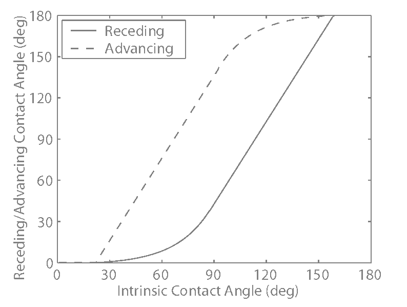
Contact angles

The keyword INIT_CONT_ANG is used to assign the contact angles for the primary drainage cycle and ALTR_CONT_ANG is used to assign the contact angles for the second (water-injection) cycle, which can be different from the primary drainage due to wettability alteration. The first argument of these keywords indicates the contact angle hysteresis model, which can be 1, 2 or 3, indicating Morrow’s contact angle hysteresis models 1 to 3. There is also an option for model 4, which is essentially same as model 3, but expects the advancing contact angles, which is particularly helpful as the advancing contact angles are what will be used in the calculations in the second (water-injection) cycle.

fig/AdvRecCA.png — Relation between advancing, receding and intrinsic contact angles in Morrow (1975) model 3.

Probability density function

The keywords INIT_CONT_ANG and ALTR_CONT_ANG and few other keywords assign a parameter, here contact angles, using a [Random, Normal or Weibull distribution. For contact angles, the distribution parameters are the second to sixth arguments of these keywords. The second argument is the smallest contact angle, the third is the largest contact angle, the fourth and fifth are the Weibull coefficients, and , and the sixth is the contact angle correlation with pore size. The correlation with pore/throat size can be rMin, rMax or rand. rMin implies smaller contact angles are assigned to smaller pores, while the rMax option leads to the opposite, and rand means no correlation to pore size. For Contact angle model 2, the seventh argument can be provided to overwrite the default separation angle (25 degrees)

If both given distribution coefficients are negative, a uniform distribution between the min and max contact angles will be used instead. Otherwise, if only the second value is negative, a normal (Gaussian) distribution will be used. Finally if both are positive, the two parameters describe the and of the truncated Weibull distribution equation:

where is a random number between 0 and 1.

snflow outputs

3D visualization and post-processing

To visualize the network and displacement process, the recommended approach is to use writeXmf keyword mentioned above, which writes .xmf files which can be opened in Paraview or in Python/gnrun for further analysis. To customise output parameters written in Xdmf format, the first option can be a combination of wk characters standing for write and keep. The rest of arguments can be either T/True or any combination of alcx characters standing for all time-steps, last time step, corners is for corners, extra-data, respectively; for example:

    #  generates Xmf visualization files
    #          write/keep   Init     OilInj   WaterFlood   Cycle3 ...;
    writeXmf:     wk        acx       lx         acx        lx

Upscaled properties

By default the code writes the computed capillary opressure, relative permeability and resistivity indices in svg files with the data embedded in a format for running further automated workflows, specifically by pylib library, or for including them into the input deck of a reservoir simulation model.

Running snflow

To run the pnflow executable, you should first generate the networks, see the documentation of pnextract executable. Then you can copy the sample input file from the src/doc folder and edit it by setting the networkFile and other keywords, described above, and run the following command in terminal or in Windows command-prompt (cmd).

snflow  input_snflow.dat

To call pnflow through SiRun, you can use the snflow input_snflow.dat command, or you can create a dictionary inline (in RAM) and pass it as the first argument of snflow command. e.g.

DictCreate inputData {
   # key: words, see above
}
pnflow  inputData

Or just use the -i argumernt of snflow to provide all the keyword inline:

pnflow  -i {
   # key: words, see above
}

References

Morrow, N. R. (1975), Effects of surface roughness on contact angle with special reference to petroleum recovery, Journal of Canadian Petroleum Technology, 14, 42-53.

Valvatne, P. H. and M J Blunt (2004), “Predictive pore-scale modeling of two-phase flow in mixed wet media,” Water Resources Research, 40, W07406

Bultreys, T., Q. Lin, Y. Gao, A. Q. Raeini, A. AlRatrout, B. Bijeljic, and M. J. Blunt (2018), Validation of model predictions of pore-scale fluid distributions during two-phase flow. Physical Review E, 97: 053104